Traditional Machine Learning

Traditional Machine Learning Overview

In this article, I will explore popular traditional machine-learning techniques at a reasonably high level. The goal is to enhance our understanding of these algorithms and provide a handy reference for future use.

Mastering traditional machine learning techniques is crucial because they provide the fundamental concepts and skills needed to tackle the complexity of advanced models like neural networks. Understanding these basics ensures a smoother transition and better performance in more sophisticated algorithms.

Contents

Supervised Learning

Supervised Learning Regression Models

Supervised Learning Classification Models

Unsupervised Learning

Unsupervised Learning Clustering models

Unsupervised Learning Dimensionality Reduction models

Time Series Econometric Models

Standard Optimization Techniques

Evaluation Metrics

Supervised Learning

Supervised learning is a machine learning technique in which a model is trained on labeled data. This means that each training example includes both the input data (independent variables) and the corresponding correct output (dependent variable). The model aims to learn the relationship between inputs and outputs to predict the output for new, unseen data accurately. Supervised learning techniques are divided into two main types: regression and classification.

For example, if you are predicting home prices, you would use a dataset that includes features such as the number of bedrooms, bathrooms, square footage, and other relevant attributes (independent variables), along with the actual sale prices of the homes (dependent variable). By learning from this labeled data, the model can predict the price of a house based on its features.

Regression Models

A regression model predicts continuous outcomes, meaning it estimates numerical values. Examples include predicting home prices or stock prices.

OLS Linear Regression

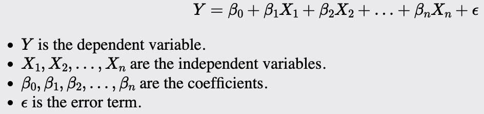
Ordinary Least Squares (OLS) Linear Regression is one of the most fundamental and widely used statistical techniques in machine learning and data analysis. It models the relationship between a dependent variable and one or more independent variables by fitting a linear equation to observed data. The primary objective of OLS regression is to minimize the sum of the squared differences between the observed and predicted values, providing the best linear unbiased estimate of the relationship.

OLS Linear Regression estimates the coefficients of the linear equation:

The Assumptions:

Linearity: The relationship between the independent and dependent variables is linear. This means that the change in the dependent variable is proportional to the change in the independent variables.
Independence: The observations are independent of each other. This implies that the value of the dependent variable for one observation is not influenced by the value of the dependent variable for another observation (i.e., no autocorrelation).
No Multicollinearity: The independent variables are not highly correlated with each other. High correlation among independent variables (multicollinearity) can make it difficult to isolate the individual effect of each independent variable on the dependent variable.
Residuals need to be IID White Noise: The residuals should be independently and identically distributed (IID) with a mean of zero and constant variance (homoscedasticity). Additionally, the residuals should be normally distributed and not exhibit autocorrelation.

Optimization:

Gradient Descent
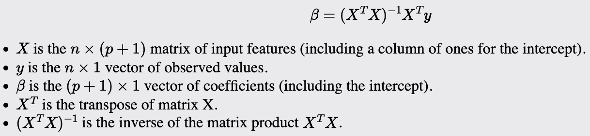
The Normal equation:

Provides a closed-form solution to solve for the coefficients (betas) that will minimize the sum of squared errors (least squares)
Computationally efficient for small to moderate-sized datasets but can be slow and memory-intensive for very large datasets due to matrix inversion.

Maximum Likelihood Estimation (MLE). It can be used but is not common.

Common Performance Metrics:

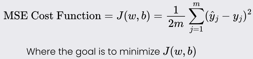
Mean Squared Error (MSE)
Root Mean Squared Error (RMSE)
R-Squared

Regularization

Ridge

Ridge regression is useful when your data has multicollinearity. It helps mitigate its effect by adding a penalty to the regression coefficients. It is also useful when you want to reduce the model complexity and prevent overfitting, especially when the number of predictors is larger than the number of observations.

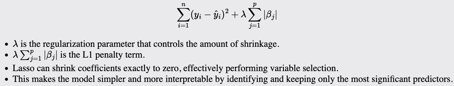
Lasso

Lasso is suitable when you want to perform both variable selection and regularization to enhance the model's prediction accuracy and interpretability. Use when you suspect that many of your predictors are not actually useful.

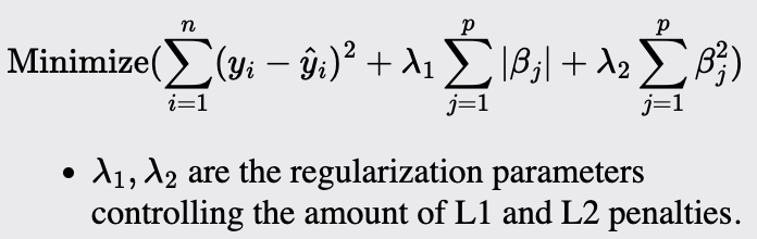
Elastic Net

Elastic Net is a hybrid of Ridge and Lasso regression that is particularly useful when multiple correlated predictors are present. It is used when Ridge's regularization strength and Lasso's variable selection capability are needed.

Decision Trees

Decision trees are useful when you need a model that is easy to interpret and visualize. They work well for both classification and regression tasks. They are particularly effective when you have a dataset with a mixture of numerical and categorical features and when the relationships between the features and the target variable are complex and non-linear.

The Method:

A decision tree splits the data into subsets based on the value of input features. This process is repeated recursively, creating a tree-like model of decisions.
At each node of the tree, the algorithm chooses the best feature and threshold to split the data based on a criterion like Gini impurity or information gain for classification and mean squared error for regression.
The process continues until the algorithm reaches a stopping criterion, such as a maximum tree depth or a minimum number of samples per leaf.

Splitting Criteria:

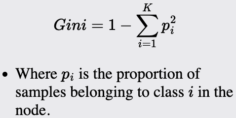
Gini Impurity: Measures the impurity of a node. Used in classification tasks.
- Notes about Gini:
  - Ranges from 0 to 1, where zero is perfect purity, and 1 indicates maximum impurity.
  - Can be interpreted as the expected error rate.
  - Sensitive to the distribution of the data
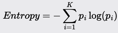
Information Gain (Entropy): Measures the reduction in entropy (randomness after a split). Used in Classification tasks.
- Notes about Entropy:
  - Ranges from 0 to log(c) where c is the number of classes.
  - Can be interpreted as the average amount of information required to determine the class of an instance.
  - It is sensitive to the number of classes
  - Entropy is more robust than Gini and tends to be less sensitive.
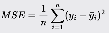
Mean Squared Error: Measures the variance within a class and is used in decision tree regression tasks.

Feature Importance: Decision trees can be used to compute the importance of features, which is the total reduction of the criterion (e.g., Gini impurity) brought by that feature. This helps understand the impact of each feature on the model's predictions.

Random Forest

Random Forests are suitable when you need a robust and accurate model that can handle both classification and regression tasks. They are particularly useful for large datasets with many features, as they help reduce overfitting, a common issue with single decision trees. Use Random Forests when you need a model that can automatically handle missing values and maintain high performance even with noisy data.

Method Overview:

They are an ensemble learning method that combines multiple decision trees to create a more accurate and stable model.

The algorithm works by constructing a large number of decision trees during training and outputting the mean prediction (for regression) or the mode of the classes (for classification).
Each tree in the forest is trained on a bootstrap sample of the original dataset, and a random subset of features is considered for splitting at each node. This randomness helps to ensure that the trees are not correlated and improves the generalization of the model.

The Method:

Create multiple bootstrap samples from the original dataset. Each sample is generated by random sampling with replacement. This means some samples will be used multiple times in a bootstrap sample, while others may not be used at all.
Grow a decision tree for each bootstrap sample. Unlike standard decision trees, each split in a Random Forest tree considers only a random subset of features. This process reduces the correlation between the trees and increases the diversity of the model.
To determine the best splits at each node in the tree, use criteria like Gini impurity or entropy for classification tasks and Mean Squared Error (MSE) for regression tasks.
Making a prediction:

For regression: The predictions from all trees are averaged to produce the final prediction.
For classification, the final prediction is based on the mode (majority vote) of the class predictions from all trees.

Gradient Boosting (XGBoost)

Gradient Boosting, specifically XGBoost, is ideal for highly robust classification and regression tasks, especially on large, complex datasets. It excels where other models, including some neural networks, might underperform. Compared to traditional boosting methods, XGBoost is excellent for handling sparse data, capturing non-linear relationships, and reducing overfitting.

Method Overview:

Is an ensemble learning method that builds models sequentially. Each new model is trained to correct the errors made by the previous models.
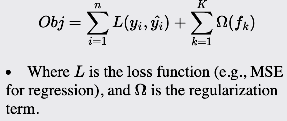
it's an optimized implementation of Gradient Boosting designed for performance and speed. It also includes regularization to reduce overfitting.

The Method:

The process starts with an initial model, often a simple model like the mean of the target values for regression or a probability score for classification.
For each subsequent model, calculate the residuals (errors) from the previous model. These residuals represent the difference between the actual values and the predicted values.
Train a new model to predict these residuals. The idea is to add this new model's predictions to the previous model's predictions to improve accuracy. In XGBoost, decision trees are typically used as the base learners. These trees are built to fit the residuals and are added to the model sequentially.
Update the overall model predictions by adding the predictions from the new model, scaled by a learning rate (shrinkage factor). This scaling helps in reducing the risk of overfitting. In classification, the predictions are typically in the form of logits or transformed probabilities.

Classification Models

A classification model predicts categorical outcomes, meaning it assigns inputs to discrete categories. Examples include identifying spam emails, classifying images of animals, or diagnosing medical conditions.

Logistic Regression

Logistic Regression is a fundamental statistical model used for binary classification tasks. It predicts the probability of a binary outcome based on one or more independent variables. Unlike linear regression, which predicts continuous outcomes, logistic regression is used to classify data into two distinct classes. It is widely valued for its simplicity, interpretability, and efficiency, making it a popular choice in various fields.

Method Overview:

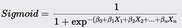
Logistic Regression models the probability that a given input belongs to a particular class. It uses the logistic function to ensure that the predicted probabilities fall within the range of 0 to 1. The model outputs a probability score, which is then thresholded to classify the input into one of the two classes.

The Method:

Define the model, specifying the independent variables that will be used to predict the binary outcome (dependent variable).
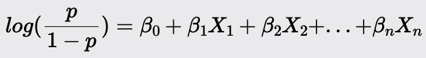
The model predicts the log odds of the positive class as a linear combination of the independent variables:
Transform the log odds into a probability using the sigmoid function
A threshold (commonly 0.5) is applied to convert this probability into a binary class prediction.

Optimization:

Maximum likelihood estimation (MLE)
Gradient Descent
Newton-Raphson Method: An iterative method that uses second-order derivatives to find the parameters that maximize the likelihood function. It converges faster than gradient descent but can be computationally intensive for large datasets.

Notes:

Assumes a linear relationship between the log odds of the dependent variable and the independent variables. It also assumes that the observations are independent.
Can be sensitive to outliers, which can affect the parameter estimates.
It assumes a linear relationship between the predictors and the log odds of the outcome. Thus, it models the decision boundary as a straight line (or a hyperplane in higher dimensions) in the transformed space of log odds, which allows it to capture linear relationships in that space.

K - Nearest Neighbor

K-Nearest Neighbors (KNN) is a simple yet powerful, non-parametric machine learning algorithm used for both classification and regression tasks. It makes predictions based on the similarity of input data points, relying on the idea that similar instances exist in close proximity to each other in the feature space.

Method Overview:

KNN predicts the output for a new data point by identifying the 'k' closest data points (neighbors) in the training dataset. For classification tasks, the predicted class is determined by the majority class among the neighbors. For regression tasks, the predicted value is the average of the values of the neighbors. The algorithm uses a distance metric, commonly Euclidean distance, to measure the similarity between data points.

The Method:

Preprocess the data; feature scaling is important because this is a distance algorithm.
Select the number of neighbors (k) to consider for making predictions. This hyperparameter needs to be chosen based on the problem.
For each data point in the test set, calculate the distance between this point and all points in the training set using a chosen distance metric.
Identify the 'k' closest data points (neighbors) in the training set based on the calculated distances.
For Classification: Determine the class of the new data point by taking a majority vote among the 'k' neighbors.
For Regression: Predict the value of the new data point by averaging the values of the 'k' neighbors.

Notes:

The value of 'k' is critical to the performance of the KNN algorithm. A small 'k' can lead to overfitting, while a large 'k' can lead to underfitting. Cross-validation is commonly used to find the optimal value of 'k.'
Standardizing the feature scales is very important. It ensures that each feature contributes equally to the prediction.

Naive Bayes

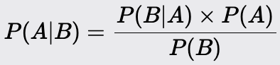
Naive Bayes is a probabilistic machine learning algorithm based on Bayes' Theorem. It is primarily used for classification tasks. Despite its simplicity, it often performs surprisingly well, especially with large datasets.

Model Overview:

It predicts the class of a given data point based on the likelihood of the features, assuming that all features contribute independently to the probability of the class. The model calculates the posterior probability of each class and assigns the class with the highest probability to the data point.

The Method:

Gather and preprocess the data
Calculate the prior probability of each class from the training data. The prior probability is the proportion of instances in each class.
Calculating the likelihoods:

Calculate the likelihood of each feature given each class. This involves estimating the probability distribution of the feature values for each class.
For categorical features, this is typically done using frequency counts. For continuous features, assumptions about the distribution (e.g., Gaussian) are made.

Use Bayes' Theorem to calculate the posterior probability of each class given the feature values of a data point:
Make predictions: For a new data point, calculate the posterior probability for each class and assign the class with the highest probability.

Notes:

Naive Bayes makes specific assumptions about the distribution of the features:

Gaussian Naive Bayes: Used for continuous features assumed to follow a normal distribution. It calculates the likelihood of a normal distribution using the probability density function (PDF). To address the issue of near-zero probabilities (which can cause computational issues), the natural log of the likelihoods is often taken.
Multinomial Naive Bayes: Suitable for discrete features, commonly used in text classification. This is the process described above, where feature occurrences are used to compute probabilities.

Smoothing Techniques: Laplace smoothing (typically denoted as alpha) can be applied to handle zero probabilities. This technique adds a small constant to all counts, ensuring that no probability is zero, which would otherwise nullify the entire probability product. This is particularly important for Multinomial Naive Bayes.
Independence Assumption: Naive Bayes is termed "naive" because it assumes that all features are independent given the class label. This means it disregards any potential order or dependency among features. For example, it treats the sequences "word1 word2" and "word2 word1" as identical, assuming no correlation between the positions of the words.

Perceptron

The Perceptron is a fundamental machine learning algorithm that serves as the building block for more complex neural networks. It is designed for binary classification tasks. As a linear classifier, the Perceptron makes predictions based on a linear combination of weights and the feature vector. You would use it when the classes can be separated by drawing a straight line or plane/hyperplane for higher dimensions.

Method Overview:

The Perceptron algorithm classifies data points by establishing a linear decision boundary (hyperplane) that separates the data into two classes. It iteratively updates the weights to minimize classification errors. If the data is linearly separable, the Perceptron algorithm will converge to a solution that correctly classifies all training instances.

The Method:

Initialize the weights and bias to small random values or zeros. The weight vector will have a size equal to the number of dimensions of the input data plus one for the bias term. These parameters will be updated during training.
For each training instance:
1. Compute the output using the current weight and bias:
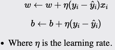
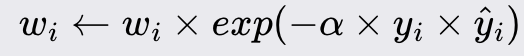
2. Update the weight and the bias if the prediction does not match the actual label:
Repeat the training step for a specified number of epochs or until the model converges (i.e., no further updates are needed).
For prediction: For a new instance, compute the weighted sum and apply the sign function to predict the class label.

Notes:

The learning rate controls the magnitude of the updates to the weights and bias. Choosing an appropriate learning rate is crucial for the algorithm's convergence. Too high a learning rate can cause the model to overshoot, while too low a learning rate can result in slow convergence.

The algorithm assumes that the data is linearly separable, meaning that a linear boundary exists that can perfectly separate the two classes. If the data is not linearly separable, the Perceptron will not converge.

Support Vector Machines (SVM)

Support Vector Machine (SVM) is a powerful and versatile machine learning algorithm for classification and regression tasks. It is known for its effectiveness in high-dimensional spaces and its ability to handle non-linear decision boundaries through kernel functions.

Method Overview:

It aims to find the optimal line/plane/hyperplane that separates the data points of different classes with the maximum margin. For non-linearly separable data, SVM uses kernel functions to transform the input space into a higher-dimensional space where a linear separator can be found.

In simpler terms, SVM is like a smart boundary drawer. Imagine you have two groups of objects on a table, and you want to draw a line to separate them. SVM finds the best line (or boundary) that not only separates the groups but also stays as far away from the closest objects in both groups as possible. This makes the separation as clear as possible. If the objects can't be separated by a straight line, SVM may square or apply another transformation to the data, making it easier to draw a separating boundary.

The Method:

Collect and preprocess the data. Feature scaling is important since SVMs are sensitive to the scales of the features.
Select a kernel function (e.g., linear, polynomial, radial basis function (RBF)).
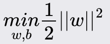
Formulate optimization problem:
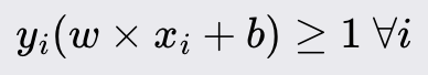
1. For classification: The goal is to maximize the margin between the support vectors.
  Subject to:
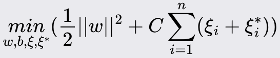
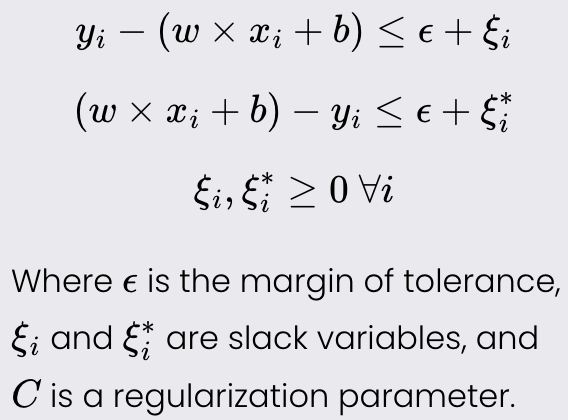
2. For regression: The goal is to find a function that approximates the target values within a tolerance margin.
  Subject to:
Solve the problem using Quadratic Programming (QP). The Lagrange multipliers are introduced to handle the constraints, resulting in the dual problem.
Making Predictions:
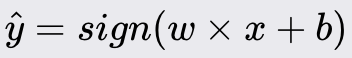
1. Classification task: For new data point x.
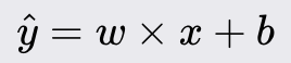
2. Regression task: For new data point x.

Notes:

It is important that the scale of the input features be uniform.
Can be computationally expensive for large datasets.

AdaBoost

AdaBoost, short for Adaptive Boosting, is an ensemble learning algorithm that combines the predictions of multiple weak learners to create a strong classifier. It is particularly effective for classification tasks but can also be adapted for regression. It works by focusing on the mistakes made by previous weak learners and adjusting the weights of the training instances to correct these errors in subsequent iterations.

Method Overview:

AdaBoost improves the accuracy of weak learners by emphasizing the training instances that are difficult to classify. Each iteration adjusts the weights of incorrectly classified instances, ensuring that subsequent weak learners focus more on these challenging cases. The final model is a weighted sum of the weak learners' predictions, where more accurate learners have higher weights.

Difference between XGBoost: While both are boosting algorithms, they differ in several key aspects. AdaBoost focuses on adjusting the weights of misclassified instances, whereas XGBoost improves the model by directly modeling the residuals (errors) from previous models. XGBoost also incorporates regularization terms in its objective function to control the complexity of the model and prevent overfitting, a feature not present in AdaBoost.

The Method: I will cover the steps for a classification problem, which is the main use of the model. However, these steps can also be modified to fit a regression problem.

Assigning equal weights to all training instances. If there are n training samples, each sample is assigned a weight of 1/n.
Train a weak learner (e.g., a decision stump; one-level decision trees) on the weighted training data.
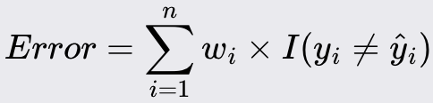
Calculate the error rate of the weak learner. The error rate is the sum of the weights of the misclassified instances:
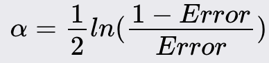
Compute the weight of the weak learner based on its error rate:
Update the weights of the training instances:
Repeat steps 2-5 for a specific number of iterations or until the error rate is sufficiently low.
The final model is a weighted sum of all weak learners:

Notes:

The model above is designed for binary classification but can be extended to multi-class problems.
AdaBoost assumes that the errors made by the weak learners are independent.

Unsupervised Learning

Unsupervised learning is a machine learning technique that trains a model on unlabeled data. Unlike supervised learning, the data does not include the correct output. The model aims to identify patterns, structures, or relationships within the data. Unsupervised learning techniques are primarily divided into two main types: clustering and dimensionality reduction.

For example, consider a dataset containing various financial metrics for a range of companies, such as revenue, profit margins, debt levels, and market capitalization, without any labels indicating the type of industry to which each company belongs. An unsupervised learning algorithm, like a clustering algorithm, can analyze these metrics and group the companies into clusters based on similarities in their financial profiles. This can help identify groups of companies with similar financial characteristics, which could be useful for tasks like sector analysis or investment strategy development.

Clustering Models

Clustering is a type of unsupervised learning that aims to group data points into clusters based on their similarities.

K - Means

K-Means is a widely used unsupervised machine learning algorithm that partitions a dataset into K distinct subsets or clusters. Each cluster is defined by its centroid, which is the mean of the points within the cluster. The goal is to minimize the variance within each cluster and maximize the variance between different clusters, thereby ensuring that the points in the same cluster are as similar as possible and those in different clusters are as different as possible.

Method Overview:

K-Means assigns each data point to one of the K clusters based on the distance to the cluster centroids. It iteratively updates the centroids and reassigns the points to clusters until the assignments no longer change or a maximum number of iterations is reached. The final result is a set of K clusters, each represented by a centroid, with the data points assigned to the nearest centroid.

The Method:

Choose K initial centroids randomly from the dataset or use a method like K-Means++ for better initial centroids.
Assign each data point to the nearest centroid based on the Euclidean distance (or another distance metric).
Calculate the new centroids as the mean of the data points assigned to each cluster.
Repeat steps 2 and 3 until the centroids do not change significantly or a predefined number of iterations is reached.

Methods for improvement:

K-Means++ improves the initialization step by spreading out the initial centroids. This helps achieve better clustering results and faster convergence.
Plot the within-cluster sum of squares against the number of clusters and look for an "elbow". That point can be used to determine the optimal number of clusters (K).
Use the Silhouette Score to measure how similar a data point is to its own cluster compared to other clusters.

Notes:

It assumes that clusters are spherical and equally sized, which might not be true for all datasets.

Scaling and normalizing the data is essential to ensure all features contribute equally to the distance calculations.

Hierarchical Clustering

Hierarchical clustering aims to construct a hierarchy of clusters without needing to predefine the number of clusters. Unlike partition-based methods such as K-Means, hierarchical clustering forms a tree-like structure known as a dendrogram. This dendrogram depicts nested groupings of data points based on their similarities, allowing for the examination of data at various levels of granularity and offering a detailed perspective on the data's inherent structure.

Method Overview:

It can be divided into two main types: agglomerative (bottom-up) and divisive (top-down).

Agglomerative Clustering: Starts with each data point as a single cluster and iteratively merges the closest pairs of clusters until all data points are in a single cluster or a stopping criterion is met.
Divisive Clustering: Starts with all data points in a single cluster and iteratively splits the clusters into smaller ones until each data point is in its own cluster or a stopping criterion is met.

The algorithm generates a dendrogram, which is a tree-like diagram that records the sequences of merges or splits. A specific number of clusters can be obtained by cutting the dendrogram at a desired level.

The Method:

Compute the distance matrix for all pairs of data points using a distance metric like Euclidean.
Create Clusters:
- Agglomerative Clustering: Start with each data point as an individual cluster.
- Divisive Clustering: Start with all data points in a single cluster.
Merge or Split Clusters:
- Agglomerative Clustering: Iteratively merge the two closest clusters based on the chosen linkage criterion (e.g., single, complete, average, or Ward's linkage).
- Divisive Clustering: Iteratively split clusters until each data point is in its own cluster.
After merging or splitting, update the distance matrix to reflect the new clusters.
Continue merging or splitting until the desired number of clusters is achieved or a stopping criterion is met.

Optimization:

Linkage: Different linkage methods affect the shape and height of the dendrogram:

Single Linkage: Minimum distance between points in different clusters.
Complete Linkage: Maximum distance between points in different clusters.
Average Linkage: Average distance between points in different clusters.
Ward's Linkage: Minimize the variance within each cluster.

The optimal number of clusters can be determined by cutting the dendrogram at various levels and evaluating the resulting clusters using metrics like silhouette score
Scaling and normalizing the data before clustering can improve the performance and interpretability of the results.
Reducing the number of dimensions using techniques like PCA can help in visualizing the clusters and improving the clustering results.

Assumptions:

Assumes that the data has an inherent hierarchical structure, which may not always be the case.
The choice of distance metric can significantly impact the clustering results. It's crucial to select a metric that aligns with the nature of the data.
The linkage method chosen affects how clusters are formed and can lead to different hierarchical structures.

Important note:

Hierarchical clustering can be computationally intensive, especially for large datasets, as it requires computing and updating the distance matrix at each step.

Gaussian Mixture Models (GMM)

Gaussian Mixture Models (GMM) are probabilistic models that assume data points are generated from a mixture of several Gaussian (normal) distributions with unknown parameters. It is widely used for clustering, density estimation, and pattern recognition. Unlike K-Means, which assigns data points to clusters rigidly, GMM provides a probabilistic approach, allowing each data point to belong to multiple clusters with certain probabilities.

Method Overview:

GMM models the data as a combination of multiple Gaussian distributions, each representing a cluster. It estimates the parameters of these Gaussian distributions (mean, covariance, and mixing coefficients) to best fit the data. The result is a soft clustering of the data, where each point has a probability of belonging to each cluster.

The Method:

Initialize: Choose the number of Gaussian components k
- Initialize the parameters of the Gaussian components:
- Means (mu) for each component k.
- Covariance matrices (sigma) for each component k.
- Mixing coefficients for each component k.
Expectation: Calculate the probability that each data point belongs to each Gaussian component k using the PDF of a normal.
Update the parameters of the Gaussian components to maximize the likelihood
Assign each data point to the Gaussian component k with the highest probability:

Optimization:

Good initialization of parameters can significantly affect the convergence and performance of GMM. Methods like K-Means clustering can be used to initialize the means of the Gaussian components.
Adding regularization terms to the covariance matrices can prevent them from becoming singular

Important Assumptions:

GMM assumes that the data within each cluster follows a Gaussian distribution.
The number of Gaussian components (clusters) must be specified in advance. Model selection techniques, such as the Bayesian Information Criterion (BIC) or Akaike Information Criterion (AIC), can help in determining the optimal number of components.
Assumes that the features are independent within each Gaussian component.
Can be computationally intensive for large datasets. Variants like mini-batch GMM can be used to improve scalability.

Dimensionality Reduction

Dimensionality reduction is a type of unsupervised learning where the goal is to reduce the number of features or dimensions in a dataset while retaining as much information as possible. This is particularly useful for visualization, noise reduction, and mitigating the curse of dimensionality in machine learning models.

Principal Component Analysis (PCA)

Principal Component Analysis (PCA) is a fundamental linear dimensionality reduction technique widely used in data analysis and machine learning. It transforms the original features of a dataset into a new set of uncorrelated features, called principal components, ordered by the amount of variance they capture from the data. It is especially useful for reducing the dimensionality of large datasets, making them easier to explore and visualize while retaining most of the significant information.

Method Overview:

PCA identifies the directions (principal components) along which the variance in the data is maximized. These directions are orthogonal (uncorrelated) and are ordered such that the first principal component captures the most variance; the second captures the second most variance, and so on. By projecting the data onto the first few principal components, PCA reduces the dimensionality of the data while preserving as much variance as possible.

The Method:

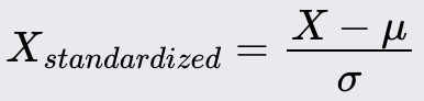
Standardize the dataset to have a mean of 0 and a standard deviation of 1. This ensures that all features contribute equally to the analysis.
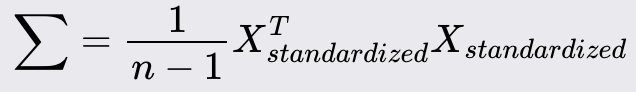
Compute the covariance matrix of the standardized data to understand how the variables vary together.
Calculate the eigenvalues and eigenvectors of the covariance matrix. The eigenvectors represent the directions of maximum variance (principal components), and the eigenvalues represent the magnitude of variance along those directions.
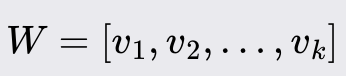
Sort the eigenvalues in descending order and order the eigenvectors accordingly. The eigenvector with the highest eigenvalue is the first principal component.
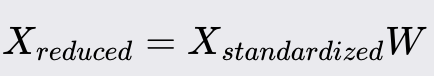
Transform the original data to the new feature space using the matrix W.

Optimization:

Create a scree plot of the eigenvalues to visualize the explained variance and identify the point where the additional components add little variance.
Use techniques like the explained variance ratio to determine the number of principal components. Typically, select the number of components that capture a desired amount of total variance (e.g., 95%).

Assumptions:

Assumes linear relationships among features.
Assumes that components with larger variance represent more significant underlying structures in the data.
The principal components are orthogonal, meaning they are uncorrelated.

Linear Discriminate Analysis (LDA)

Linear Discriminant Analysis (LDA) is a supervised dimensionality reduction technique commonly used in machine learning for both classification and feature extraction. It aims to find a linear combination of features that best separates two or more classes of objects or events. LDA is particularly effective when the data distribution is Gaussian, and classes have similar covariance structures.

Method Overview:

LDA projects the data onto a lower-dimensional space in a way that maximizes the separation (discrimination) between the different classes. It does this by maximizing the ratio of between-class variance to within-class variance, ensuring that the classes are as distinct as possible in the new feature space.

The Method:

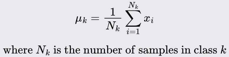
Compute the mean of each class:
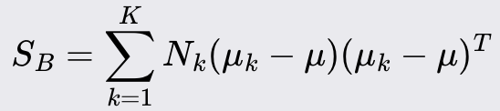
Calculate the scatter matrix for each class and sum them up:

Calculate the scatter matrix that represents the spread between the mean vectors of the classes.
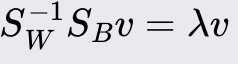
Solve the eigenvalue problem:
Sort the eigenvectors by their eigenvalues in descending order and select the top k, eigenvectors to form the matrix W.
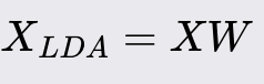
Project the original data onto the new feature space using the matrix:

Optimization:

Regularize the scatter matrices to handle cases where S_SW is singular or nearly singular.

Assumptions:

The data for each class is normally distributed.
All classes have the same covariance matrix.
Relationships between features are linear.

Autoencoders

I wanted to highlight autoencoders because, although they are not a traditional machine learning approach, they are a powerful tool for reducing the complexity of large, intricate datasets.

Autoencoders are a type of artificial neural network used for unsupervised learning, primarily for dimensionality reduction, feature learning, and data reconstruction. An autoencoder consists of two main parts: the encoder and the decoder. The encoder maps the input data to a lower-dimensional latent space while the decoder reconstructs the original data from this latent representation. The goal is to learn a compressed representation of the data that can be used to accurately reconstruct the input.

Method Overview:

The algorithm learns to compress (encode) the input data into a lower-dimensional representation and then decompress (decode) it back to its original form. By minimizing the difference between the original input and the reconstructed output, autoencoders effectively learn meaningful features of the data.

Time Series Models

These are statistical methods designed to analyze and predict data points collected or recorded at specific intervals. They capture the temporal (time) dependencies and patterns within the data, making them essential for forecasting future values.

AutoRegressive (AR) Models

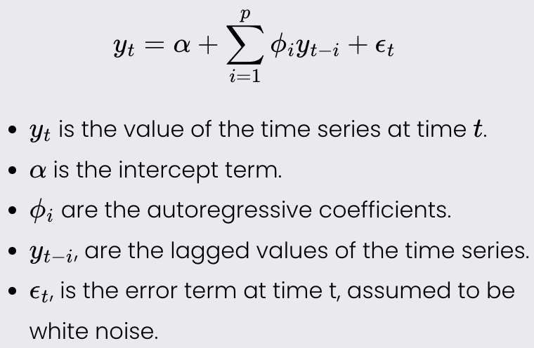
Autoregressive (AR) models are a type of time series model used to predict future values based on past values. AR models assume that the current value of the time series is a linear combination of its previous values and a stochastic error term. These models are particularly useful for analyzing and forecasting stationary time series data, where statistical properties such as mean and variance remain constant over time.

Method Overview:

AR models use past observations to predict future values. The idea is that past values contain information about future values, and by identifying the relationships between these past values, the model can make accurate predictions.

The Method:

Choose the order *p* of the AR model, which is the number of lagged observations to include. This is often determined using criteria such as the Akaike Information Criterion (AIC), the Bayesian Information Criterion (BIC), or by examining the Autocorrelation Function (ACF) plot to identify the significant lags.
The AR(p) model can be written as:
Estimate the parameters using methods such as Maximum Likelihood Estimation.
Evaluate the residuals (the differences between the actual and predicted values) to check for patterns or correlations that would indicate a poor fit (white noise).

Optimization:

Use information criteria such as AIC or BIC to select the optimal order of the AR model.
Ensure data fits the assumptions below.

Assumptions:

The time series must be stationary, meaning its statistical properties do not change over time. This can often be achieved through differencing or detrending the data.
The relationship between the current value and its past values must be linear.
The error term should be white noise, meaning it has a constant mean and variance and is not autocorrelated.

Moving Average (MA) Models

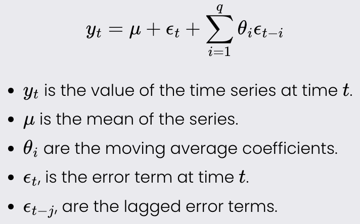
Moving Average (MA) models are a type of time series model used to predict future values based on past forecast errors. Unlike Autoregressive (AR) models, which rely on past values of the time series, MA models use past error terms to make predictions. These models are particularly useful for modeling time series data that exhibit noise or random shocks.

Method Overview:

These models express the current value of the time series as a linear combination of past forecast errors. By modeling the dependencies on past errors, MA models can effectively capture the short-term correlations in the data, making them useful for smoothing and forecasting.

The Method:

Choose the order q of the MA model, which is the number of lagged forecast errors to include. This can be done by using criteria such as the Akaike Information Criterion (AIC), the Bayesian Information Criterion (BIC), or by examining the Autocorrelation Function (ACF) plot to identify the significant drops in the lags.
The MA(q) model can be written as:
Estimate the parameters mu and theta using methods such as Maximum Likelihood Estimation (MLE).
Evaluate the residuals (the differences between the actual and predicted values) to check for patterns or correlations that would indicate a poor fit.

Optimization:

Use AIC or BIC to select the best order q.
Apply cross-validation to determine the robustness of the model.

The assumptions are the same as an AR process.

Autoregressive Moving Average (ARMA) Models

Autoregressive Moving Average (ARMA) models combine the properties of Autoregressive (AR) models and Moving Average (MA) models to analyze and predict time series data. These models use past values and past forecast errors to predict future values, making them powerful tools for modeling stationary time series data. By incorporating both autoregressive and moving average components, ARMA models can capture a wide range of temporal dependencies in the data.

Method Overview:

ARMA models predict future values of a time series by expressing the current value as a linear combination of past values (autoregressive part) and past forecast errors (moving average part). This dual approach allows ARMA models to handle various patterns in the data, including trends and noise.

The Method:

Choose the orders p and q of the ARMA model, where p is the number of lagged observations in the autoregressive part and q is the number of lagged forecast errors in the moving average part. This can be determined using criteria such as the Akaike Information Criterion (AIC) or the Bayesian Information Criterion (BIC).
The ARMA(p, q) model can be written as:
Estimate the parameters alpha, phi, and theta using methods such as Maximum Likelihood Estimation (MLE).
Evaluate the residuals (the differences between the actual and predicted values) to check for patterns or correlations that would indicate a poor fit.

The Assumptions and optimization techniques are the same as an AR or MA process.

Generalized Autoregressive Conditional Heteroskedasticity (GARCH)

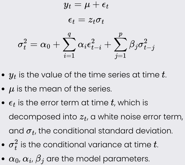
Generalized Autoregressive Conditional Heteroskedasticity (GARCH) models are used in time series analysis to model and forecast the volatility of financial returns. Unlike traditional time series models that assume constant variance, GARCH models account for changing variance over time, which is a common feature in financial time series data. This makes these models particularly useful for risk management and financial market analysis.

Method Overview:

These models estimate the current volatility of a time series based on past observations and past forecast errors. The basic idea is that large changes tend to be followed by large changes, and small changes tend to be followed by small changes, indicating volatility clustering. GARCH models capture this by modeling the variance of the time series as a function of past variances and past forecast errors.

The Method:

Choose the orders p and q of the GARCH(p, q) model. Here, p is the number of lagged conditional variances, and q is the number of lagged squared residuals (past forecast errors).
The GARCH(p, q) model can be written as:
Estimate the parameters mu, alpha_0, alpha_i, and beta_j using Maximum Likelihood Estimation (MLE).
Evaluate the residuals and conditional variances to check for patterns or correlations that would indicate a poor fit.

The assumptions, and optimization techniques for GARCH models are largely similar to those used in AR and MA processes. However, a key distinction for GARCH models is that the conditional variance must always be positive because variance cannot be negative.

Common Optimization Techniques

Gradient Descent

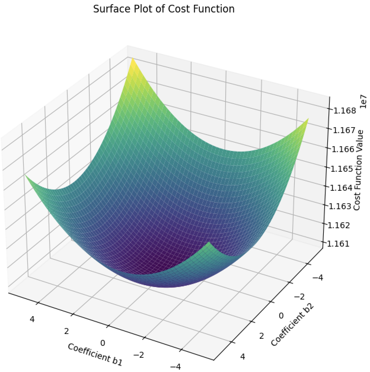
Goal: minimize a cost function of a given model. The cost function tells you how well your model fits your data for a given set of weights and bias.

Example: Linear Regression cost function

The Method:

Start with an initial guess for weights and bias term.
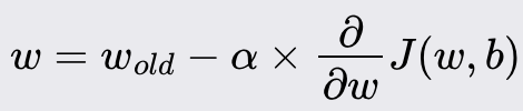
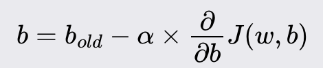
Iteratively update weights and bias, reducing the cost function
- New weight value:
- New bias value:
  - Alpha is the learning rate. i.e., how large of a step you take downhill. It’s between 0 and 1, typically about 0.001
You continue to update weights and bias until a threshold is met, typically a number of iterations or until there is little change between steps.

The Three Types of Gradient Descent:

Stochastic Gradient Descent: The gradient is computed and updated using a single training example at a time. This method produces a lot of noise, although it can more easily escape local minima.
Mini Batch Gradient Descent: is a compromise between Stochastic Gradient Descent and Batch Gradient Descent. The gradient is computed and updated using a small random subset (mini-batch) of the training data. You need to define the batch size.
Batch Gradient Descent: The gradient is computed and updated using the entire training dataset. This approach ensures that the direction of the gradient is more accurate, leading to more stable convergence. However, it requires more memory and computational power.

Important Notes:

You need to update weights and bias terms simultaneously
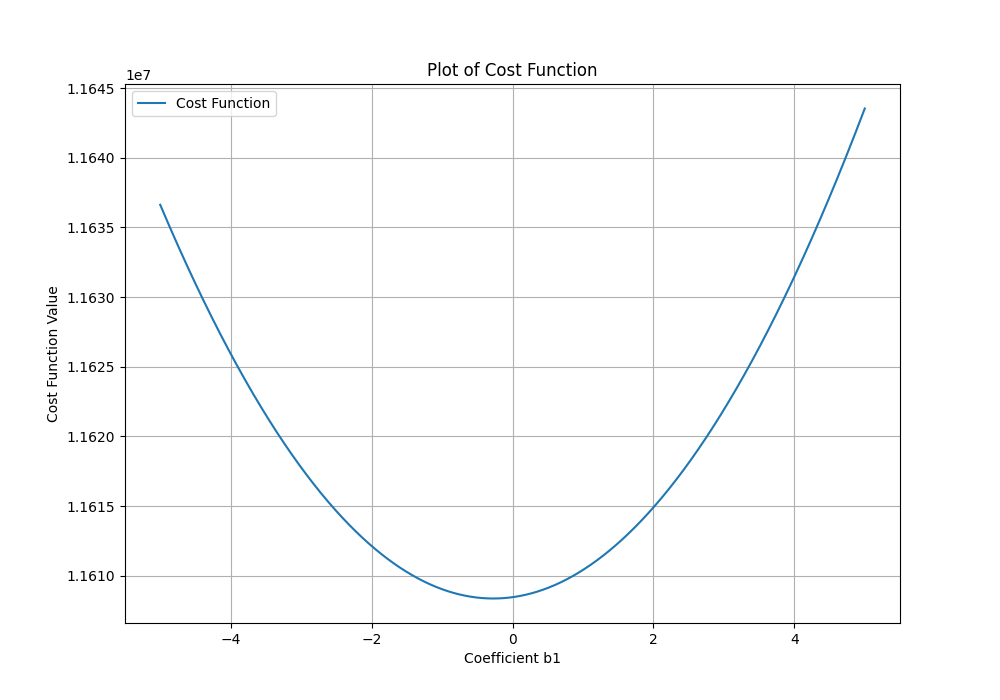
If the cost function is not a squared error cost function, then the surface of the function may look like hilly terrain. In this case, you may get stuck in local minima.
If alpha is too small or large, convergence may take a long time, or it may never happen because you overshoot the minima.
Scaling your independent variables will increase the convergence rate.
To check if things are working correctly, plot the cost function against the number of iterations. It should always be decreasing.

Bonus Point: The ADAM optimizer; Builds upon gradient descent by incorporating two additional factors: momentum and RMSProp. Momentum accelerates the gradient descent by considering past gradients to smooth out updates, while RMSProp adapts the learning rate for each parameter based on recent gradient magnitudes.

Advantages: It is able to reduce noise in updates and adjust the learning rate during convergence.

Disadvantage: Requires some hyperparameter tuning

Maximum Likelihood Estimation (MLE)

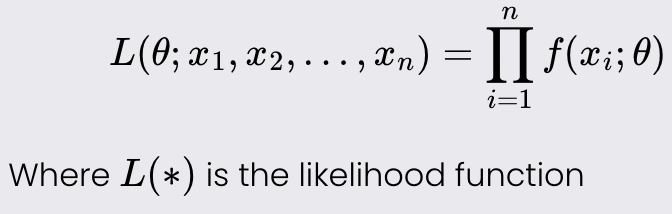
Goal: Maximize the likelihood function to find the parameter values that best explain the observed data. The likelihood function measures how likely it is to observe the given data given a set of parameters in a statistical model.

Notes:

The likelihood function depends on the underlying distribution that your data follows (E.g., Gaussian, Poisson, Binomial, etc.).
The likelihood function is equal to the joint probability distribution function or joint probability mass function.
Determining the correct underlying distribution is crucial; failing to do so can result in biased or inconsistent parameter estimates.
Larger sample sizes provide better estimates and ensure your sample estimate is close to the true population parameter.
Akaike Information Criterion (AIC) or Bayesian Information Criterion (BIC) can be used to compare models fitted via MLE.

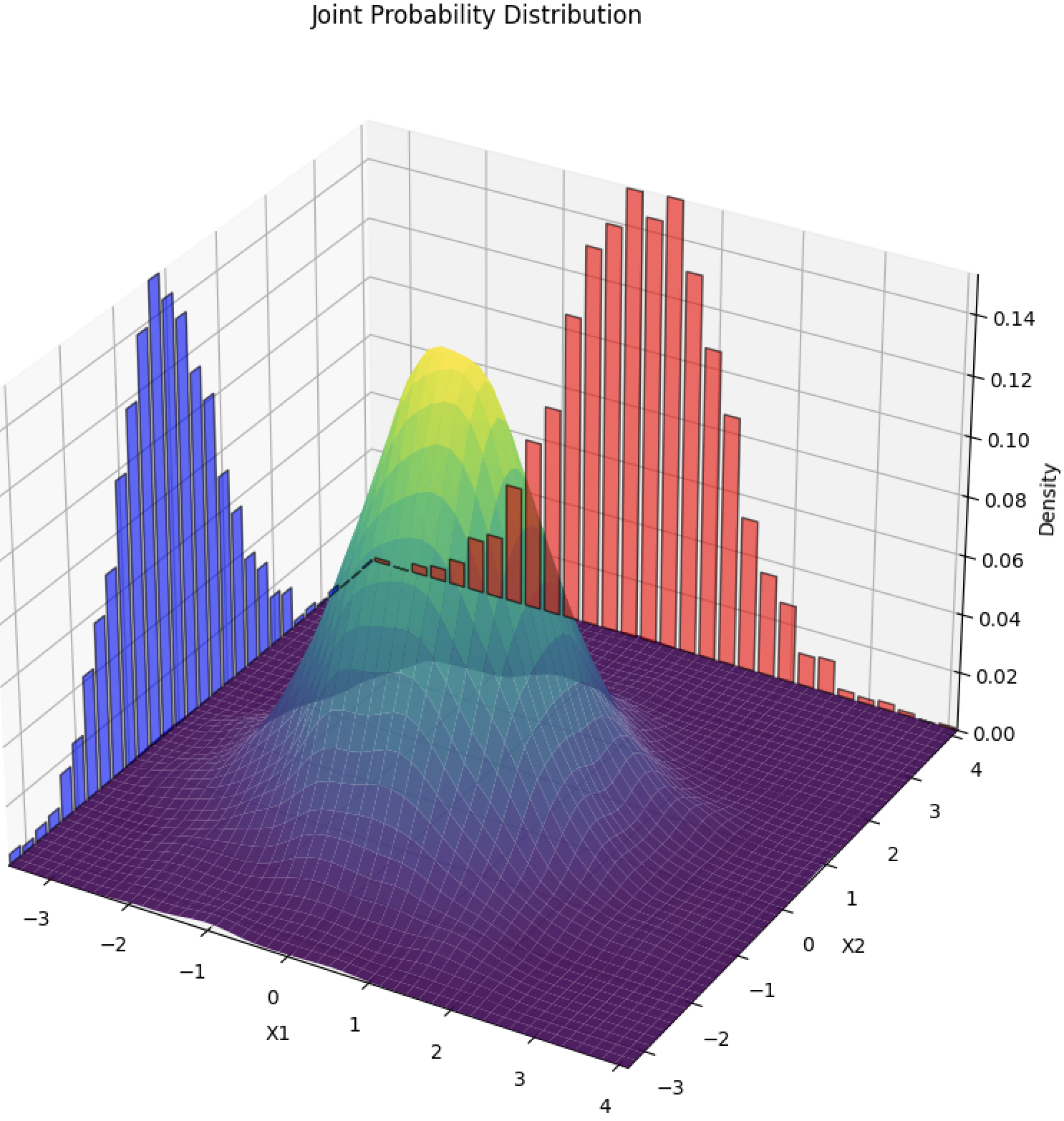
Joint Probability Distribution: describes the likelihood of two or more random variables occurring simultaneously. For discrete variables, it gives the probability of specific combinations of values, like a table showing the chances of different outcomes for two dice rolls. For continuous variables, a probability density function is used to indicate how likely different combinations of values are. This distribution helps understand the relationship and dependence between multiple variables by considering their combined behavior.

Mathematically, if f(*) is the probability density function (pdf) or probability mass function (pmf) of a single observation given parameters theta, the joint probability distribution for n independent observations is:

The Method:

Identify the probability distribution that best fits your data and determine its probability density function (PDF).
Use the PDF to write the likelihood function, which represents the joint probability distribution of the observed data given the parameters.
Take the natural logarithm of the likelihood function to obtain the log-likelihood function, turning products into sums for simpler calculations.
Differentiate the log-likelihood function with respect to the unknown parameters.
Set the derivatives to zero and solve the resulting system of equations to find the parameter estimates that maximize the likelihood function.
These steps will give you the parameter values that make the observed data most probable under the chosen distribution! Yay

Performance Metrics

For Regression Problems

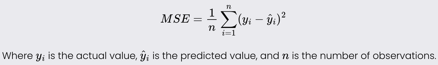
Mean Squared Error

Mean Squared Error is a measure of the average squared difference between the actual and predicted values. It is used to evaluate the accuracy of a regression model.

Lower values of MSE indicate better model performance as it signifies smaller errors.

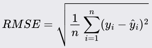
Root Mean Squared Error (RMSE)

Root Mean Squared Error is the square root of the Mean Squared Error. It provides the error magnitude in the same unit as the original data.

Like MSE, lower values of RMSE indicate better model performance.

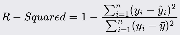
R - Squared

R -Squared is a statistical measure that represents the proportion of the variance for the dependent variable that's explained by the independent variables in a regression model.

Values range from 0 to 1. Higher values indicate a better fit, with 1 indicating perfect prediction.

For Classification Problems

Accuracy

Accuracy is the proportion of correctly predicted instances (both true positives and true negatives) out of the total instances evaluated.
Higher accuracy indicates better performance, with 1 being perfect accuracy.

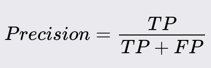
Precision

Precision is the ratio of correctly predicted positive observations to the total predicted positives.

High precision indicates that most of the predicted positives are true positives.
Precision is particularly important when the cost of false positives is high. For example, in spam detection, a false positive (marking a legitimate email as spam) can result in important emails being missed.

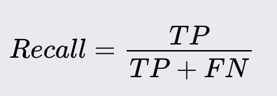
Recall

Recall (Sensitivity) is the ratio of correctly predicted positive observations to the total number of actual positive observations.

High recall indicates that most of the actual positive cases are correctly identified.
Recall is crucial when the cost of false negatives is high. For instance, in cancer diagnosis, a false negative (failing to diagnose a patient with cancer) can have severe repercussions, as it may delay necessary treatment.

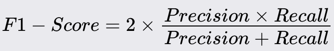
F1 - Score

F1 Score is the weighted average of Precision and Recall. It considers both false positives and false negatives.

Higher F1 score indicates better balance between precision and recall.

AUC - ROC

AUC-ROC is a way to measure how well a classification model can distinguish between classes. The ROC curve shows the trade-off between true positive rate and false positive rate at different thresholds, and the AUC (Area Under the Curve) tells us how well the model separates the

A higher AUC means the model is better at distinguishing between positive and negative classes, with 1 being perfect and 0.5 being no better than random guessing.